The problem posed in the basic study of integration is to find for the graph of a particular function  , the area under the curve of
  between two points. As seen here:
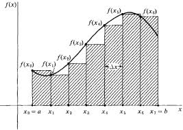
The process is to take a set of intervals  along a segment of the x-axis, and treat each such interval as the base of a rectangle, with the value for
  as the height of our rectangle, then summing each rectangle allows us to calculate the approximate area under the curve. An increase in exactitude can be achieved as we reduce the base of each rectangle so that “intuitively” no rectangle exceeds or “dips” under the height of the curve .
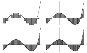
As can be seen here the rectangles can extend above and below the x-axis, but the result is the same the smaller we set the base of our rectangles, the more accurately we approximate the space between the axis and the curve. So at first glance this technique seems merely about calculating an area  . Formally we denote this as follows:
Let  be two points on the x-axis and , then we divide the segment as follows:

and we set  as before. Now to calculate the area of those rectangles we need to define the summation of the products:

But this will be inexact unless we shrink the base of these rectangles i.e.  as described above. To achieve this last specification we simply take the limit of as
  approaches zero. This process is called integration. Formally:


More specifically this is a definite integral since we have specified the bound but we need not. If instead we treat the bounds as variable then we still have a function known as the indefinite integral.
The Summation/Difference Property:
We want to show that:
![\int\limits_{a}^{b} [f(x) + g(x)] \Delta x = \int\limits_{a}^{b} f(x) \Delta x + \int\limits_{a}^{b} g(x) \Delta x](https://s0.wp.com/latex.php?latex=%5Cint%5Climits_%7Ba%7D%5E%7Bb%7D+%5Bf%28x%29+%2B+g%28x%29%5D+%5CDelta+x+%3D+%5Cint%5Climits_%7Ba%7D%5E%7Bb%7D+f%28x%29+%5CDelta+x+%2B+%5Cint%5Climits_%7Ba%7D%5E%7Bb%7D+g%28x%29+%5CDelta+x&bg=ffffff&fg=666666&s=0&c=20201002)
but this is almost self evident as we can see:
![\lim_{\Delta \to 0} [ \sum\limits_{i}^{n} f(x_{i}) \Delta x] + \lim_{\Delta \to 0} [ \sum\limits_{i}^{n} g(x_{i}) \Delta x ]](https://s0.wp.com/latex.php?latex=%5Clim_%7B%5CDelta+%5Cto+0%7D+%5B+%5Csum%5Climits_%7Bi%7D%5E%7Bn%7D+f%28x_%7Bi%7D%29+%5CDelta+x%5D+%2B+%5Clim_%7B%5CDelta+%5Cto+0%7D+%5B+%5Csum%5Climits_%7Bi%7D%5E%7Bn%7D+g%28x_%7Bi%7D%29+%5CDelta+x+%5D&bg=ffffff&fg=666666&s=0&c=20201002)
is by the distributive properties of limits equivalent to:
![\lim_{\Delta \to 0} [ \sum\limits_{i}^{n} f(x_{i}) \Delta x] + [ \sum\limits_{i}^{n} g(x_{i}) \Delta x]](https://s0.wp.com/latex.php?latex=%5Clim_%7B%5CDelta+%5Cto+0%7D+%5B+%5Csum%5Climits_%7Bi%7D%5E%7Bn%7D+f%28x_%7Bi%7D%29+%5CDelta+x%5D+%2B+%5B+%5Csum%5Climits_%7Bi%7D%5E%7Bn%7D+g%28x_%7Bi%7D%29+%5CDelta+x%5D&bg=ffffff&fg=666666&s=0&c=20201002)
but by distribution and rearranging we get:

![[f(x_{i}) + g(x_{i})] \Delta x](https://s0.wp.com/latex.php?latex=%5Bf%28x_%7Bi%7D%29+%2B+g%28x_%7Bi%7D%29%5D+%5CDelta+x+&bg=ffffff&fg=666666&s=0&c=20201002)
which is exactly:
![\int\limits_{a}^{b} [f(x) + g(x)] \Delta x](https://s0.wp.com/latex.php?latex=%5Cint%5Climits_%7Ba%7D%5E%7Bb%7D+%5Bf%28x%29+%2B+g%28x%29%5D+%5CDelta+x&bg=ffffff&fg=666666&s=0&c=20201002)
as desired. An exactly analogous proof applies to show that  distributes over the difference of two functions.
The Mean Value Theorem(s):
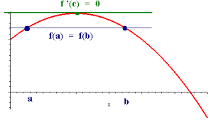
First note that for any continuous function there is a maximum and minimum point on the interval i.e. there exists a point at the lowest or highest depth of the curve. Now suppose is defined in the closed interval ![[a. b]](https://s0.wp.com/latex.php?latex=%5Ba.+b%5D&bg=ffffff&fg=666666&s=0&c=20201002) and is differentiable in the open interval
and is differentiable in the open interval  , we will show that if
  , then there is a point
  such that
  This result is known as Rolle’s Theorem.
There are three cases (i) where  is defined as a constant function with value
  and the limit of a constant function collapses to 0 at all points, so this would prove the theorem.
If on the other hand (i)  or (ii)
  then there is slightly more work to be done. There are two sub-cases but both are analogous so we prove (ii): Suppose , then pick a point
  such that
  . This satisfies the hypothesis so it remains to show that We do this by reductio, but first we prove a small lemma.
Lemma: If f'(p) is positive (negative) then f is increasing(decreasing) at a neighborhood of p.
Assume positive (the negative case is analogous), then we know by work here that the the limit of the quotient minus the derivative is equivalent to 0, so rewriting in terms of  can take any
  and see that:

When  Let
Let  , then add
  to all sides to get:
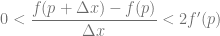
which ensures that the difference quotient is positive, and both numerator and denominator must have the same sign. It falls out that:  . Hence is an increasing function in the neighborhood around p. This completes the proof.
Rolle’s Theorem
To complete Rolle’s theorem we need only consider the case that  , either
  is positive or negative, and then by the above lemma, is either decreasing or increasing in the continuous p-neighborhood. In either case M would not be the maximum or extreme point on the interval. This is a contradiction. Hence
  as desired. An analogous strategy works for the case (i). Geometrically this theorem states that the slope of the curve vanishes at some point in the interval between
  and
and  , which means the slope becomes briefly horizontal as can be seen in the picture above.
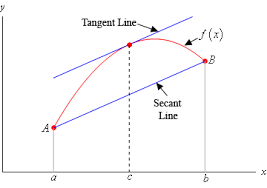
The Mean Value Theorem (Differentiation)
Let be continuous in the closed interval [a, b ] and differentiable, with the derivative  in the open interval (a, b). Then there is a point c in (a, b) such that:

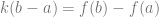
This can be most intuitively thought of as saying that if tracks movement of an object across a plane between two points a and b, then there is a point on it’s trajectory of the function’s equivalent to the average rate of ascent. If you travel between A and B 100 miles apart and arrive in an hour, then at some point on your journey you were traveling at one hundred miles an hour. Here the claim is that the instantaneous rate of change at point c is the same as the average rate of change between the two points a and b. Geometrically it means that the slope of the curve at some point must match the slope of the secant line.
The Proof:
Define a function  , where k is a constant so that
  Hence,
  . We can solve for . Take

adding  to each side we get:

subtracting  becomes:


from which it follows:

which is equivalent to:
then dividing by  and canceling we get:
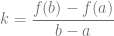
ensuring that k is equivalent to the slope of the secant line. We must show that there is a the tangent line on the curve of equivalent to k, if we are to prove the mean value theorem. That is we must find a point  such that
But then note that since  satisfies the hypothesis of Rolle’s theorem, so we have a point
  Differentiating we see that
![g'(c) = [f'(c) - (k c')] = 0](https://s0.wp.com/latex.php?latex=g%27%28c%29+%3D+%5Bf%27%28c%29+-+%28k+c%27%29%5D+%3D+0&bg=ffffff&fg=666666&s=0&c=20201002)
but the derivative c is 1 so this collapses into
![g'(c) = [f'(c) - k(1)] = 0](https://s0.wp.com/latex.php?latex=g%27%28c%29+%3D+%5Bf%27%28c%29+-+k%281%29%5D+%3D+0&bg=ffffff&fg=666666&s=0&c=20201002)
from which we can infer that

so we have shown that an appropriate point exists as desired.
The Mean Value Theorem: Integration
We want to prove that if is continuous in the closed interval [a, b], then there is a point ![c \in [a, b]](https://s0.wp.com/latex.php?latex=c+%5Cin+%5Ba%2C+b%5D&bg=ffffff&fg=666666&s=0&c=20201002) such that
such that
We begin the proof by letting m and M be defined as the minimum and maximum points on the curve as in the last proof. We are looking for the average value of our integrand function defined on the the interval [a, b ]. First let:

then since

it follows:

which by definition and distribution is just:

then taking the limit as approaches zero adds nothing, so:

then dividing by  we get:
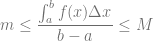
which is equivalent to:

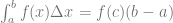
Let’s call this point ![f(c) \in [m, M].](https://s0.wp.com/latex.php?latex=f%28c%29+%5Cin+%5Bm%2C+M%5D.&bg=ffffff&fg=666666&s=0&c=20201002) Then by the intermediate value theorem (proof easy and omitted), there is a point . Geometrically the mean value theorem for integrals can be understood as stating that for any area under the curve of the line there is a rectangle defined at the average height
Then by the intermediate value theorem (proof easy and omitted), there is a point . Geometrically the mean value theorem for integrals can be understood as stating that for any area under the curve of the line there is a rectangle defined at the average height  with respect to [a, b] such that the area of it is equivalent to the area under the total curve defined by . In a picture:

The area in excess of the height is “compensated” for by inclusion of the novel sections defined by our rectangle. To see this precisely: note that ![[ \dfrac{1}{b-c} \int_{a}^{b} f(c) \Delta c]\dfrac{b-c}{1}](https://s0.wp.com/latex.php?latex=%5B+%5Cdfrac%7B1%7D%7Bb-c%7D+%5Cint_%7Ba%7D%5E%7Bb%7D+f%28c%29+%5CDelta+c%5D%5Cdfrac%7Bb-c%7D%7B1%7D&bg=ffffff&fg=666666&s=0&c=20201002) cancels to give us
cancels to give us  as desired. This concludes the section; in the next post we will prove the first fundamental theorem of calculus.

Pingback: Some Facts about Famous Functions | Aspiring PI